Insight, 35,15-22 , 1992.

The Classification of weld defects from ultrasonic images: a neural network approach

C G Windsor, F Anselme, L Capineri and J P Mason Addresses and biographies are at the end of the paper.

Abstract:

Neural networks are shown to be effective in being able to distinguish crack-like weld defects from more benign volumetric defects by directly analysing the images collected from ultrasonic scanning. The performance is similar to that of existing methods based on extracted feature parameters. In each case around 94% of the defects in a database derived from 84 artificially-produced defects of known type are placed correctly into one of four classes: rough and smooth cracks, slag and porosity. However, the methods based on classification directly from the ultrasonic image are faster, and the speed is sufficient to allow on-line classification during data collection. A prototype based on the Harwell ZIPSCAN ultrasonic scanning system is described.

Figure 1:A typical scanning system for detecting defects within a weld using an ultrasonic probe. Pulses of ultrasound are emitted by the probe and reflected from the defect, possibly after reflection from the back wall. The reflected sound is measured as a function of time to give the defect range, knowing the sound velocity

1. Introduction

The inspection of large welded components such as pressure vessels and pipes often requires the collection of data from hundreds of metres of weld, followed by a rigorous characterisation to detect significant defects. This characterisation is at present performed largely by human operators; often after the data collection from the weld has been completed. The human eye is unparalleled in its ability to recognise significant patterns after a period of suitable training and experience. However, even the best operators suffer from fatigue and loss of concentration, so human error cannot be neglected. An automated characterisation offers the possibility of an impartial, standardised performance 24 hours a day.

In this paper we discuss how neural networks may be used to assist in the automation process, by providing a rapid and accurate characterisation of a number of different defect types. In section 2 we consider the problem in general, defining the different classes of defect considered in this study, the conventional approach of feature extraction, and how neural networks may find application in this area. Section 3 presents a comparison of neural networks with a number of classical techniques for classifying feature extraction data. The results of such comparisons suggest that the best opportunity for neural networks lies in their potential to analyse the data at an earlier stage, prior to feature extraction.

A series of comparisons is presented in section 4 where it is argued that a number of direct approaches are able to match the success rates achieved through the feature extraction, whilst offering a potential for on-line detection by virtue of their high speed of operation. The demonstration of an on-line system is described in section 5 and its development in the future is discussed in section 6. We draw some final conclusions in section 7.

2. Automatic Defect Characterisation during Ultrasonic Inspection

2.1 Weld defects

Ultrasonic data from welds are frequently collected from transducers emitting and receiving pulses of ultrasound in a directional beam at one or more angles to the inspection surface (see for example Figure 1). In an automatic data collection system, recordings are made of the reflected ultrasound signal intensity as a function of time - the "A" scan. Spatial scans are then generally made perpendicular to the weld length. This set of A scans forms a two-dimensional pattern of intensity as a function of range (depth) and position (stand-off distance from the weld centre), known as a "B" scan. Often sets of these B scan images are made at intervals along the length of the weld, and at various probe angles.

Any defect which is present in the material will reflect the ultrasound in a pattern characteristic of its type. The four types considered in this study are illustrated schematically in Figure 2. They are:

(i)Rough cracks. These are the most dangerous defects. They generally lie close to a plane, but have irregular facets which reflect ultrasound from several angles.

(ii)Smooth cracks. Such cracks, or lack of fusion defects, act as planar reflectors and reflect ultrasound only near the angle for specular reflection.

(iii) Slag inclusions. Slag inclusions are point-like and reflect sound from any angle.

(iv)Porosity. Porosity comprises many point-like defects, which again reflect sound from any angle.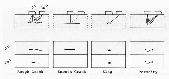

Figure 2:Schematic diagrams of the types of weld defect considered in this work. The upper part of the figure shows the beams reflected (full lines) and not reflected (dashed lines) by each defect. The lower part of the figure shows the generic form of the images at the two angles

Figure 2 also indicates an idealised ultrasonic image which might be expected from each defect type. In differentiating the defect types it should be noted that another important aspect is the position of the defect with respect to the geometry of the weld. Smooth cracks are likely to be aligned parallel to the weld metal interface, whereas rough cracks are most often found near the weld root. Slag and porosity are only found within the weld metal volume.

Consideration of the physical characteristics which typify the defect type can play a key part in the classical approach to the present problem. This approach consists of extracting suitable features from the complex ultrasonic signals, and using these feature values as input to a classifier. The application of this technique to weld defect characterisation is discussed further in the next section.

2.2 Characterisation by feature extraction

Trained human operators characterise defects from the general appearance of the patterns from probes with different angles, and the calculated position of the defect with respect to the weld. Each pattern is different, but the human eye, or rather the human brain, is readily trained to observe "features", or distinctive characteristics of each class.

Extensive work has been performed by Burch and his co-workers⁽¹⁾⁽²⁾ to perform defect classification automatically from features extracted from sets of B scans carried out along a weld at 2 or 3 different probe angles. Such data can be processed into a pattern of reflected ultrasound intensity as a function of four different parameters: depth; stand-off distance; position along the weld; and probe angle.

Burch et al collected a series of 112 such ultrasonic images from welds in which defects of a defined type had been artificially induced. It was found that the data from these images could be accurately classified on the basis of the values of four extracted features:

(i) Amplitude: the ratio of the signal intensity at high and low angles - low for smooth cracks.

(ii) Kurtosis: related to the spread of the signal in depth - high for rough cracks and porosity.

(iii) Sphericity: the deviation of the defect from a plane - high for porosity.

(iv)" KM" related to the spread in the reflected signal amplitude with ultrasound angle.

For classification purposes a Bayes classifier was used⁽³⁾ in which each defect type was assumed to give rise to a Gaussian probability distribution in the four-dimensional feature parameter space. As only a small dataset was available to be used for both training and testing, a "leave-one-out" method was adopted in which all but one of the points was used as the training set, and the excluded point was used as a test point. This was repeated with each point in turn being left out whilst a running total of the success rate was maintained. In such testing on the present problem, a 100% success rate could be achieved.

2.3 Classification using neural networks - a new opportunity

The idea of mimicking the way in which the brain behaves in order to carry out the sort of tasks at which humans are particularly skilled is not new. In the 1940s, Hebb and others correctly saw the brain, not as a single computer, but as a network of independent computational elements, the neurons, each of which operates in parallel to form a collective tool of great power.

In the 1980s an explosion of activity took place as it became clear that artificial neural networks of quite modest size could perform powerful computational tasks such as face and speech recognition. Suitable reviews of the whole field are available ⁽⁴⁾ Here we briefly introduce the type of neural network used in the present application to classify defect types from the multi-dimensional images measured by ultrasonics. In this application the neural net may be used merely as a classifier of suitable features extracted by classical methods, or it may be used for the more complex task of analysing the raw image data, and so incorporating the feature extraction process.

Figure 3 illustrates the analogy between the way the eye might classify an ultrasonic image and the way an artificial neural network might do the same task. The eye scans the image by sweeping its focus, the fovea, over the image and passes it along the optic nerve to the retina where the image analysis occurs. Layers of neurons receive the image and relay the signals simultaneously to many of the neurons in the following layer. Each of these neurons evaluates a new signal which in turn is passed on to the neurons in the following layer. In some way, not yet fully understood, each layer serves to pick out increasingly abstracted features of the image. The final process is a perception by us of a classification.

Figure 3. An ultrasonic image as seen by the eye and by an artificial neural network. In the eye, as the image is scanned, the optic nerve passes it to the visual cortex for analysis, where layers of neurons act as feature detectors which pass on signals from which a decision is made. The receptive field MLP model is very similar; the field is swept over the image, and the excitation level of each pixel is fed to each of several hidden units, which again act as feature detectors

The most widely used artificial neural network, the multilayer perceptron (MLP) mimics the layered structure of the retina by supposing a few layers of neurons, each of which is fully connected to those in the next layer. The fovea may be modelled by a receptive field, which is scanned across the image. The signals from the pixels in the receptive field are fed simultaneously to the second layer of neurons, the "hidden units". Each neuron sums the inputs from each pixel, after multiplication by "weights" representing the strengths of the connections between neurons. These neurons behave essentially independently, switching to a level defined by the weighted input signal and in turn feeding signals to other neurons. The hidden units act as "feature detectors" which respond to some common characteristic of a set of images. The activation values of the neurons in the final layer, the "output units", are used to define the classes being distinguished. For example one neuron may be allocated to turn on for a crack defect whilst another is activated when a slag defect is presented as input.

The network, as thus defined, reflects at a very crude level our knowledge of how biological systems respond to external stimuli. What is less clear is how to copy the human's ability to learn from experience: How do we derive the values of the weights which connect the neurons, since these are what determine the response of the network for any given input image? To date the approach has been to set the weights during a 'training' phase in which a suitable algorithm is allowed to adjust the weights in such a way that over the set of images used for training, the output units respond as closely as possible to the class of defect of the image.

The error back propagation method of Rumelhart et al ⁽⁵⁾ defines one algorithm for training the network. It is an iterative procedure involving the repeated presentation of each image in the training set to the input units, propagation of the signals forward to calculate a set of output signals, and then propagation back of an error signal (a measure of the difference between the actual and desired output). This signal is then used to adjust each weight in a direction guaranteed to reduce the overall error.

Error back propagation is computationally intensive, although improved optimisation techniques, such as conjugate gradient methods, mean that very much faster and more robust results can now be achieved compared with the original gradient descent algorithm proposed by Rumelhart et al. Moreover, once trained, the network can classify a new pattern in a single forward pass through the network, which may take only a few computational cycles. In an application such as defect characterisation, the training need be learned only occasionally. In the main task of classification the network need only operate in the fast, forward propagation mode.

The back propagation method has no biological justification but it certainly acts as a powerful statistical classification algorithm for non-linear mapping of some input image into classes. The biological "cycle time" is some tens of milliseconds, and the human eye can indeed classify in a few tens of this cycle time. The promise of neural networks is that, implemented in silicon, and using parallel computational techniques, the classification can be performed in a few tens of a cycle time of nanoseconds.

Neural networks may also be used in a conventional way to classify ultrasonic images on the basis of extracted features ^(6)(7)(8) rather than from the raw image data. More recently expert systems have also been used to apply rule-based methods to extracted features ⁽⁹⁾. Before exploring the use of neural networks for image classification we shall therefore first see how they compare in performance with conventional classifiers when dealing with extracted feature data.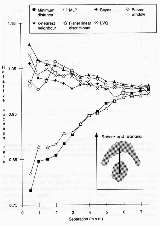

Figure 4:The success rate for classification of test points belonging to one of the two (a spherical and a banana-shaped) probability distributions illustrated. The relative performance of each classifier is plotted as a function of the distance between the centres of the two distributions

3. A Comparison of Neural Network and Conventional Classifiers

3.1 Generic studies Project ANNIE (Applications of Neural Networks for Industry in Europe) was carried out as part of the European Community's ESPRIT 2 programme, and had as one of its objectives the comparison of neural network with conventional classifiers ⁽¹⁰⁾ In order to make such comparisons of general applicability, studies were made of the performance of a variety of classifiers on artificially generated generic datasets whose properties - such as dimensionality, cluster shape, cluster overlap and number of examples - could be varied at will.

The choice of cluster shapes was guided by experience of the sort of feature space distributions found commonly in realistic problems, such as a spherical cluster representing one class and a banana-shaped cluster representing another. A suitable parametric description of each of these two distributions was defined with the probability density falling off in a Gaussian fashion as the distance from the class centre increased. Data was generated by sampling points randomly according to these probability distributions. By varying the separation of the means of these two clusters, different datasets could be produced in which the difficulty of obtaining accurate classification could be controlled as required.

The performance of a variety of different classifiers (for descriptions see ⁽¹¹⁾ for the conventional methods, ⁽¹²⁾ for learning vector quantisation (LVQ) and ⁽⁵⁾ for the MLP using error back-propagation) are shown in Figure 4. At large separations, there is little overlap between the clusters so the problem is easy. At closer separations the sphere may lie within the arc of the banana shape. Although the class overlap is still low, to be successful any classifier must be able to generate a curved decision boundary.

Certain classifiers, such as the minimum distance and Fisher linear discriminant methods are constrained to produce linear boundaries; these perform badly at small class separation, whilst others which have no such linear constraint - such as the k- nearest neighbour method - continue to perform well. However, when the degree of overlap becomes very large the k-nearest neighbour method develops an inappropriate convoluted boundary around particular training points and its performance degrades. The MLP using error back-propagation can similarly overfit the training data if applied with too many adjustable weights.

3.2 Real feature data

We also examined the performance of the different classifiers on the real feature space data obtained as described above in section 2. (Note, however, that the earlier data of reference ⁽¹⁾ was used for which there were only 66 defects and the KM feature parameter was not available. This meant that it was not possible to achieve the 100% success rate obtained in reference ⁽²⁾. Figure 5 shows the success rates obtained as a function of the inverse of the fraction of the dataset used for training. Many of the classification methods contain parameters, which could be varied to obtain an optimum classification, and methods such as the k-nearest neighbour method performed well at low fractions. The MLP method was generally good over the whole range⁽¹³⁾.

3.3 Conclusions

The clear conclusion that emerged from the studies of both generic and real feature data was that several appropriately chosen methods, both conventional and neural network, were able to give very similar results when presented with the same data. An MLP can describe the arbitrary boundaries between the clusters in feature space, but so can the Parzen window and k-nearest neighbour methods. Performance is more closely related to the degree by which the information in the data matches the complexity of the classifier. An MLP or learning vector quantisation approach must be tuned so that the number of adjustable weights is appropriately less than the number of features in the training set. It can be argued that this ad hoc approach is little better than other parametric methods. A clear potential advantage of neural network methods in general is their speed in carrying out classification. In the present case, however, such an advantage is not important, so the methods appear to offer no critical advantage in performance over the best choice of conventional methods for classification of features in a few dimensions.

Figure 5:The success rate for classification of real feature parameter ultrasonic data of weld defects as determined by several classifiers as a function of the fraction of the dataset used for training

4. Characterisation from Ultrasonic Images

While the feature extraction method described above has been shown to give good results for characterising ultrasonic defect images, the computation of the feature parameters can be complex and provide a bottle-neck to implementation of an on-line system. Another drawback is that the determination of optimum features can require a considerable amount of study and must be repeated for each type of problem tackled.

To counter these disadvantages, further studies within the ANNIE project considered whether the ultrasonic image data could be used directly as the input to neural network and other adaptive learning methods. The hope was that the labour in deciding the best features would be eliminated since the training process itself would pick out those combinations of data from the image which are characteristic of each class. Unfortunately, when treating the entire image as the input space each example becomes a single point in a high dimensionality feature space in which each pixel is a feature. The problem is that trivial changes to the image which make no difference to the defect characterisation, such as a translation by one pixel, will result in a change to every feature value and break up any obvious is clustering of classes.

A naive approach in which the complete image is used as the input to an MLP is therefore unlikely to be successful, especially if only comparatively few example images are available for training; the network would need to learn that transforms such as translation of the image should have no effect on the classification, and would need to create wildly complex decision boundaries. To stand any chance of being successful, it is therefore necessary to build in suitable prior knowledge about valid transformations, so that the neural network learning can be focussed on distinguishing genuinely different features between image types of each class.

4.1 Characterisation of artificial generic images

The first stage of evaluating the direct approach was made with artificially generated images, designed to mimic the type of problems encountered with real ultrasonic images. Figure 6 shows some of the images used. Arbitrary numbers of these images could be readily generated, but to represent the likely number of real examples which would be available, we limited the numbers to 40 images for training and 160 for testing. A variety of conventional methods were compared, including template matching, a moment expansion and an adaptive receptive field.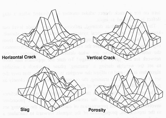

Figure 6: Artificially generated images designed to mimic ultrasonic data from four classes of defect. Large datasets of such images could be generated with variable defect sizes, shapes, spreads, statistical noise and background level

Template Matching

The template matching method consisted of averaging the images of every example of the same defect type in the training set (having first translated the images so that their centres of gravity were in the same position). The test images were compared with each of the defect templates, and the template giving the lowest least squares deviation determined the defect type.

Moment Expansion

The moments method consists of evaluating the x and y radii of gyration of the image intensity about its centre of gravity. Vertical cracks have a low x-axis radius, but a high y-axis one; the reverse is true for horizontal cracks. Slag defects have low radii in both directions, and porosity high radii in both directions. Thus, in principle, a classification can be made from these two radii alone using a simple classifier such as k-nearest neighbour.

Adaptive Receptive Field Method

Receptive field methods are closely allied to biological vision systems in which fovea sweep across a scene and respond to standard parts of images. They are based on defining suitable filters (small scale images) which can be scanned across the image under investigation. The response or activation of the receptive field at any particular position is then given by the correlation of the filter with the underlying image, and a maximum activation can be found which located that part of the image which is most similar to the receptive field.

To determine the optimum receptive field for each defect type we adopted an iterative, adaptive procedure in which an initially random field was swept across images of one defect type. At the position of maximum activation, some fraction of the underlying image was added to the filter in a pixel-by-pixel fashion. This was done repeatedly until a stable field resulted. Classification of test images was achieved by sweeping the receptive field of each defect type across the image and seeking the maximum overall activation.

Neural Network Methods

For comparison purposes three neural network based methods with supervised learning were also investigated: a fully connected MLP network; a hybrid method incorporating a receptive field which provided inputs to an MLP network, "and a special variant of an MLP network in which tolerance to translation is built in by ensuring that the weights in layers of the network are common - shared weights network method (see for example ⁽¹⁴⁾).

In the receptive field MLP method, portions of the images around the defect centre of gravity were presented as training images to an MLP network whose number of inputs equalled the number of pixels in the receptive field. With an output unit for each of the defect classes, the network could be trained by supervised learning. In testing, the receptive field was swept over the image and the class determined from the output giving the largest excitation.

The shared weights method is a related, but more powerful, algorithm in which the full image is presented to a back propagation network, but where constraints on the weights ensure that the response of the network is invariant to the position in the image at which a characteristic feature occurs.

Comparison of Results

The results obtained with each method are summarised in Table 1. The conclusion was that direct image classification was indeed possible and that both adaptive conventional methods and appropriate neural networks could be used. As expected, "direct" methods of simple template matching or input to large MLP networks performed badly. However methods based on a "receptive field" swept across the image proved relatively successful, and this was clearly due to the invariance of their response to translations of the image. The results with generic images gave us the confidence to tackle direct characterisation on real image with the most promising methods. This is described in the next section.

Table 1: The best results for classifiers of generic images

Method	Field size	No. Hidden units	Success rate training	Success rate testing
Template matching	-	-	75.0%	50.6%
Moments	-	-	59.0%	54.4%
Adaptive receptive field	5x5	-	97.5%	98.1%
MLP	-	3	100.0%	78.1%
Shared weights MLP	5x5	8	100.0%	96.8%
Receptive field + MLP	5x5	4	100.0%	91.8%

Figure 7: Processed ultrasonic images from typical defects of each type. The data are shown as grey levels as a function of position in three dimensions and at two angles

4.2 Direct classification of real images

The real ultrasonic images from the datasets collected by Burch were characterised by the adaptive receptive field and MLP receptive field methods described above. The original data contained rectified images from some 66 defects and were available to us as images of around 0.5 mm resolution in depth, 1 mm resolution in stand-off distance and 2 mm resolution along the weld, and at two different probe angles.

The images were first preprocessed to obtain coarser images of uniform size centred on the centre of gravity of the defect. This made them suitable for direct input to a neural network. Figure 7 shows data from typical defects of each type expressed as a grey level image in three dimensions and two angles. The processed image size was 7x7x7x2pixels.

The adaptive receptive field method gave the best results with quite small receptive fields, typically just 3x3x3x2 pixels long the depth, distance from weld, distance along weld and angle axes respectively. This size of receptive field gives 54 adjustable parameters to the classifier, very much less than the number of pixels in the training data, so that the problem of overfitting is much reduced. A success rate of 93.9% was achieved on a leave-one-out basis. This result was not appreciably dependent on the fraction of the dataset used for training. Figure 8 shows the form of the adaptive receptive field after 4 iterations when convergence was essentially complete.

The receptive field back propagation method also gave good results for small receptive field sizes. With a field of 3x3x3x2 pixels and four hidden units, the network has some 232 adjustable weights and does not seem susceptible to overfitting with the present set of 66 receptive field images of 54 pixels each. The leave-one-out performance was 94% with 4 hidden units. A shared weight network containing four receptive fields each of size 5x5x5x2 gave 90% success in a leave-one-out analysis of the dataset.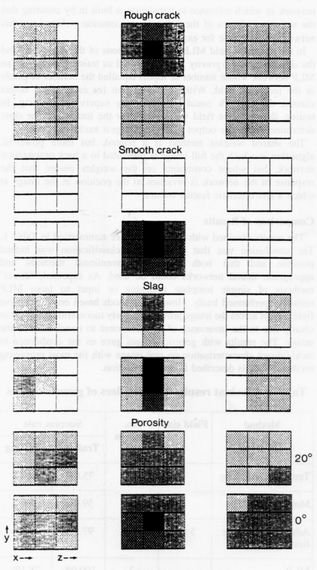

Figure 8: The trained adaptive receptive fields for each of the four defect classes. Each field consists of a grey-level image as a function of depth into the weld (z), stand-off distance from the weld (x), distance along the weld (y) and the angle of ultrasound beam. The characteristics of each class given schematically in Figure 2 may be seen in each image

The best results obtained from three-image classification and three feature based methods are summarised in Table 2. (Note that the feature and image datasets used in this comparison are largely derived from the same set of ultrasonic scans; however, because of difficulties experienced in recovering all the image data, the feature-based dataset does contain a few more examples than the image dataset.)

The results of Table 2 show that comparable performance can be achieved with a range of methods, both classical and neural net, and both feature-based and image-based. It was also found that whenever misclassification did occur in either the feature-based or image-based approaches, they tended to be the same ones. This indicates a possible difficulty in assigning correct labels to the training set associated with the subjective input of even a well-trained human observer.

Given this slight ambiguity as to the absolute performance levels of all the methods, we concluded that in taking the methods forward to the next step of on-line classification, we should choose the approach on the basis of other factors such as speed of operation, ease of implementation and flexibility in use. The image-based methods are, at present, significantly faster in execution and were therefore chosen. Of these the neural net-based methods are particularly fast in classifying inputs, although the MLP networks do have the drawback of requiring significant training times. This drawback is, of course, ameliorated by the fact that the training normally needs to be performed only once, and so its impact on practical operation is not significant.

Table 2: Performance of different classifiers in the -characterisation of real ultrasonic data

Method	Basis	Type	Parameters of the method	Success rate
k-nearest neighbour	Features	Conventional	-	91.6%
Weighted minimum distance	Features	Conventional	k=3	94.4%
Direct MLP	Features	Neural network	4 hidden units	94.0%
Adaptive receptive field	Image	Conventional	3x3x3x2	93.9%
Receptive field + MLP	Image	Neurall network	3x3x3x2 field: 6 hiden units	93.9%
Shared weights MLP	Image	Neural network	4 off 5x5x5x2 receptive field	90.0%

Figure 9: The on-line defect characterisation system based on the ZIPSCAN ultrasonic data collection. The probe is to the bottom right of the picture, and is being scanned over the plate containing a single "V" weld

5. An On-line Demonstrator for Defect Characterisation

At the end of the ANNIE project, defect characterisation was chosen as one of the ideas which would be taken forward to a demonstration stage. A demonstrator, illustrated in Figure 9, was built into the Harwell "ZIPSCAN" ultrasonic data collection system ⁽¹⁵⁾ This system consists of a pair of probes which measure ultrasonic reflections at two angles: 60 and 45 degrees. (These probe angles were chosen because the angle of the V-weld under study was about 60 degrees; the beam of the first probe was therefore perpendicular to the weld/metal interface after reflection off the back wall.) A B-scan can be collected by scanning the probes along a direction perpendicular to a weld sample. The weld plate can then be moved perpendicularly to the scan direction so that the complete four-dimensional scan used in the earlier part of the project is collected. The system is controlled by a Digital Equipment Corporation LSI 11/73 computer. The new software was incorporated into the existing menu system and provides an on-line characterisation of any defect following the scan.

Figure 10 shows an example of the reflected ultrasound intensity from a rough crack defect. It is stored in a compressed format allowing a resolution of around 1 mm in stand-off distance (x), 0.4 mm in range (z), and 2 mm in length along the weld (y). Each facet of the crack gives rise to an angled streak representing the change in the range of the reflection as the probe is moved. The crosses represent the computed centre of gravity of the defect.

The upper portion of Figure 11 shows the image of Figure 10 processed to give a standard sized image of resolution 2x2x4 mm suitable for classification. The image has been centred so that the r +re of gravity of the defect lies on the central pixel of the image, has been rotated so that the z-axis lies perpendicular to the weld interface. The facets of the rough crack now appear at roughly constant values of z. Two classifiers were included in the demonstrator; an adaptive receptive field and a receptive field MLP method. In both cases the receptive fields were trained off-line on a separate system and down-loaded onto the ZIPSCAN system through a floppy disk. The lower part of Figure 11 shows the trained adaptive receptive fields for the four classes of defects. The white rectangles in the upper part of the figure show the position in the image where the match with the rough crack receptive field was best.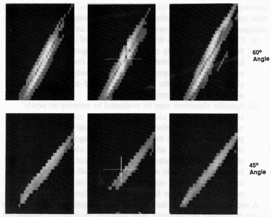

Figure 10: An ultrasonic image from a rough crack as measured on the on-line defect characterisation system. Each box represents a B scan with range (z) shown vertically and stand-off distance (x) shown horizontally. Different distances along the weld (y) are presented across the page. The upper set are measured at 60 ^o and the lower set at 45^o. The rough crack shows up as diagonal streaks from each facet of the crack, reflected into both angles. The crosses denote the centre of gravity of the image

Although the on-line system gave reliable results for some types of defects - particularly smooth lack-of-fusion cracks, its performance is not yet equal to that from the carefully collected datasets used in the earlier part of project ANNIE. Future developments will assess how the performance can be improved by examining the influence of experimental uncertainties such as the contact probe coupling factor, the different efficiency of the probes as well as the distance dependent attenuation of the ultrasound. Extending the number of probe angles to three is also under consideration.

6. Discussion

The work described above leads us to believe that it will be possible to develop a commercial on-line flaw detection system in the near future. A PC-based system such as the HFD2, which has been developed at Harwell, should be a suitable vehicle for incorporating new modules for defect characterisation as extensions to the basic ultrasonic data collection system. Two options can be considered:
(i) Classifiers based on the existing dataset of ultrasonic images from welds. In many respects these encapsulate the same knowledge an experienced tester obtains from years of experience. They represent a valuable resource for characterisation of the four types of weld defect considered within the ANNIE project analysis.
(ii) Specific classifiers may be evaluated by training on newly collected data. The characterisation may concentrate on whatever type of defect is considered most important for the problem in hand. In this case the advantages of both direct image analysis, and adaptive learning are clear. The highly skilled research needed to choose the most appropriate feature parameters is no longer needed; all that is required is supervised learning computation which can extract the required information from the newly collected data. A second way in which the new methods can greatly increase safety is by presenting the operator with displays designed to exploit his judgement and experience as much as possible. For example, our display of the compressed data, with optimum resolution for a neural network analysis, is often more readily characterised by the human eye than is possible by looking through the several pages of original high resolution B scans at different positions and angles. When the data is transformed into real space variables and superimposed on a diagram of the weld geometry the operator is able to bring new factors into account. For example a defect aligned along the weld interface is likely to be a lack-of-fusion smooth crack. Porosity is likely to lie within the bulk of weld metal. Thus a system should be able to give the operator both an on-line characterisation and also a display to enable him to confirm the decision. A reliability factor could also be introduced so the operator could be given a "NOT CLASSIFIED" output. If there was any doubt in the classification, the option would be available for the scan to be repeated at higher resolution or over a different area. Such options are not possible if the data analysis is performed off-line.

Figure 11: The processed image from the rough crack of Figure 10. The image has been further averaged, and a rotation of the image made so that the depth axis is perpendicular to the weld interface. The receptive fields for each of the four classes are shown at the bottom of the figure. White rectangles show the positions in the image where the rough crack receptive field has its best match

7. Conclusions

Neural networks and classical classifiers have been applied to the problem of defect characterisation from ultrasonic data. Success rates of order 90% have been obtained from a variety of methods. Those based on direct analysis of the image give results comparable with those based on expertly chosen features. They avoid the extensive computations necessary in feature extraction, and the expert labour needed to choose appropriate features to tackle any new characterisation problem. Adaptive learning methods, based on processed training images of three-dimensional data taken at two angles, have been incorporated successfully into an on-line demonstrator. Both an adaptive receptive field and a neural network MLP classifier have given good results.

8. Acknowledgements

The authors are grateful to the Commission of the European Community for financial support for the ANNIE project, and, both before and after this, the support of the Corporate Research Programme of AEA Technology. One of us (LC) acknowledges the support of a fellowship from the British Council whilst he worked at Harwell's National NDT Centre during 1991.

9. References

1. Burch S F and Bealing N K. NDT International 19(3), 145-153. 1986.

2. Burch S F, Lomas A R and Ramsey A T. Brit J NDT 32(7), 347-350. 1990.

3. Duda R O and Hart P. "Pattern Classification and Scene Analysis", John Wiley, New York. 1973.

4. Lippmann R P. IEEE ASSP Magazine 4. 1987.

5. Rumelhart D E and McClelland J L, eds "Parallel Distributed Processing", Vols 1 and 2, MIT Press. 1986.

6. Baker A R and Windsor C G. NDT International 22(2), 97-105. 1989.

7. Windsor C G. Neural Networks from Models to Applications ed L Personnaz, G Dreyfus, IDSET, Paris, 592-601. 1989.

8. Song S J and Schmerr L W. Rev Prog in Quantitative Nondestructive Evaluation, 104, 697-703. 1991.

9. McNab A and Dunlop I. Brit J NDT 33(1), 11-18. 1991.

10. Croall I F and Mason J P, eds "Industrial Application of Neural Networks. Project ANNIE Handbook", to be published by Springer-Verlag. 1992.

11. Tou J T and Gonzalez R C. "Pattern Recognition Principles", Addison-Wesley. 1974.

12. Kohonen T. "Self-Organisation and Associative Memory", Springer-Verlag. 1988.

13. Geman F, Bienenstock E and Doursat R. Neural Computation, Vol 4, pp 1-58. 1992

14. Guy on I, Albrecht P, Le Cun Y, Denker J and Hubbard W in Proc Int Neural Network Conf, Paris, 42-45. 1990.

15. Smith B J. Brit J NDT 28(1), 9-16. 1986.

Authors biographies

Colin Windsor is a Senior Scientist in the National Nondestructive Testing Centre at AEA Technology, Harwell. He worked in Materials Science for many years before becoming interested in neural network applications some 5 years ago. He is an Honorary Professor of Physics at Birmingham University.

Francois Anselme worked at Harwell on attachment from the University of Paris. His attachment was supported by Electricite de France. He has worked on the analysis of eddy currents using neural network.

Dr Lorenzo Capineri worked at Harwell on attachment from the Ultrasound and NDT Laboratory, in the University of Florence.

Dr John Mason leads the Neural Network Applications Group at AEA Technology's Harwell Laboratory. Trained as a nuclear physicist, he now manages a group which concentrates on developing industrial applications of neural networks.

Presented at the 31st Annual British Conference on NDT, Cambridge, September 1992.